Distances between elements (standardized)
Source:vignettes/web/elements-distances-standardized.Rmd
elements-distances-standardized.RmdIntroduction
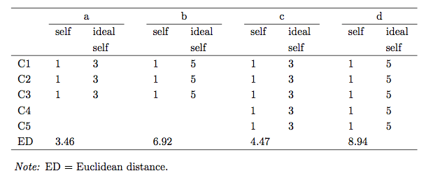
As a similarity measure in grids different types of Minkowski metrics, especially the Euclidean and city-block metric are frequently used. The Euclidean distance is the sum of squared differences between the ratings on two different elements. They are, however, no standardized measure. The distances strongly depend on the number of constructs and the rating range. The figure below demonstrates this fact. Note how the distance changes although the rating pattern remains identical.
In order to be able to compare distances across grids of different size and rating range a standardization is desireable. Also, the notion of significance of a distance, i.e. a distance which is unusually big, is easier with a standard reference measure. Different suggestions have been made in the literature of how to standardize Euclidean interelement distances (Hartmann, 1992; Heckmann, 2012; Slater, 1977). The three variants will be briefly discussed and the corresponing R-Code is demonstrated.
Slater distances (1977)
Description
The first suggestion to standardization was made by Slater (1977). He essentially calculated an expected average Euclidean distance for the case if the ratings are randomly distributed. To standardize the grids he suggested to divide the matrix of Euclidean distances by this unit of expected distance . The Slater standardization thus is the division of the Euclidean distances by the distance expected on average. Hence, distances bigger than 1 are greater than expected, distances smaller than 1 are smaller than expected.
R-Code
The function distanceSlater calculates Slater distances
for a grid.
distanceSlater(boeker)
#
# ##########################
# Distances between elements
# ##########################
#
# Distance method:  Slater (standardized Euclidean)
# Normalized:
#                                1    2    3    4    5    6    7    8    9   10   11   12   13   14   15
# (1) self                  1      1.03 0.75 0.69 0.87 1.19 0.80 1.03 0.99 0.59 1.79 0.58 0.55 0.64 0.54
# (2) ideal self            2           1.11 0.78 1.06 1.31 1.07 0.97 1.14 0.97 1.56 1.22 1.21 1.24 1.25
# (3) mother                3                0.73 0.53 0.95 0.55 0.81 0.64 0.67 1.58 0.69 0.83 0.77 0.69
# (4) father                4                     0.63 1.15 0.65 0.90 0.83 0.69 1.66 0.84 0.91 0.98 0.89
# (5) kurt                  5                          0.89 0.57 0.79 0.57 0.72 1.51 0.79 0.93 0.87 0.83
# (6) karl                  6                               0.94 0.74 0.66 1.09 0.97 1.17 1.22 1.08 1.15
# (7) george                7                                    0.92 0.65 0.81 1.51 0.73 0.91 0.92 0.78
# (8) martin                8                                         0.68 0.80 1.27 1.09 1.10 1.01 1.07
# (9) elizabeth             9                                              0.87 1.31 1.00 1.13 1.03 0.98
# (10) therapist           10                                                   1.74 0.65 0.63 0.69 0.65
# (11) irene               11                                                        1.83 1.86 1.72 1.84
# (12) childhood self      12                                                             0.43 0.50 0.34
# (13) self before illness 13                                                                  0.43 0.41
# (14) self with delusion  14                                                                       0.45
# (15) self as dreamer     15
#
# Note that Slater distances cannot be compared across grids with a different number of constructs (see Hartmann, 1992).
You can save the results and define the way they are displayed using
the print method. For example we could display distances
only within certain boundaries, using the cutoff values
.8 and 1.2 to indicate very big or small
distances as suggested by Norris and Makhlouf-Norris (1976).
d <- distanceSlater(boeker)
print(d, cutoffs = c(.8, 1.2))
#
# ##########################
# Distances between elements
# ##########################
#
# Distance method:  Slater (standardized Euclidean)
# Normalized:
#                                1    2    3    4    5    6    7    8    9   10   11   12   13   14   15
# (1) self                  1           0.75 0.69           0.80           0.59 1.79 0.58 0.55 0.64 0.54
# (2) ideal self            2                0.78      1.31                     1.56 1.22 1.21 1.24 1.25
# (3) mother                3                0.73 0.53      0.55      0.64 0.67 1.58 0.69      0.77 0.69
# (4) father                4                     0.63      0.65           0.69 1.66
# (5) kurt                  5                               0.57 0.79 0.57 0.72 1.51 0.79
# (6) karl                  6                                    0.74 0.66                1.22
# (7) george                7                                         0.65      1.51 0.73           0.78
# (8) martin                8                                         0.68 0.80 1.27
# (9) elizabeth             9                                                   1.31
# (10) therapist           10                                                   1.74 0.65 0.63 0.69 0.65
# (11) irene               11                                                        1.83 1.86 1.72 1.84
# (12) childhood self      12                                                             0.43 0.50 0.34
# (13) self before illness 13                                                                  0.43 0.41
# (14) self with delusion  14                                                                       0.45
# (15) self as dreamer     15
#
# Note that Slater distances cannot be compared across grids with a different number of constructs (see Hartmann, 1992).
Calculation
Let be the raw grid matrix and be the grid matrix centered around the construct means, with , where is the mean of the construct. Further, let
The Euclidean distances results in:
For the standardization, Slater proposes to use the expected Euclidean distance between a random pair of elements taken from the grid. The average for and would then be where is the number of elements in the grid. The average of the off-line diagonals of is (see Slater, 1951, for a proof). Inserted into the formula above it gives the following expected average euclidean distance which is outputted as unit of expected distance in Slater’s INGRID program.
The calculated euclidean distances are then divided by , the unit of expected distance to form the matrix of standardized element distances , with
Hartmann distances (1992)
Description
Hartmann (1992) showed in a Monte Carlo study that Slater distances (see above) based on random grids, for which Slater coined the expression quasis, have a skewed distribution, a mean and a standard deviation depending on the number of constructs elicited. Hence, the distances cannot be compared across grids with a different number of constructs. As a remedy he suggested a linear transformation (z-transformation) of the Slater distance values which take into account their estimated (or alternatively expected) mean and their standard deviation to standardize them. Hartmann distances represent a more accurate version of Slater distances. Note that Hartmann distances are multiplied by -1 to allow an interpretation similar to correlation coefficients: negative Hartmann values represent an above average dissimilarity (i.e. a big Slater distance) and positive values represent an above average similarity (i.e. a small Slater distance).
The Hartmann distance is calculated as follows (Hartmann, 1992, p. 49).
Where denotes the Slater distances of the grid, the sample distribution’s mean value and the sample distributions’s standard deviation.
R-Code
The function distanceHartmann calculates Hartmann
distances. The function can be operated in two ways. The default option
(method="paper") uses precalculated mean and standard
deviations (as e.g. given in Hartmann
(1992)) for the standardization.
distanceHartmann(boeker)
# | | | 0% | |= | 0% | |= | 1% | |== | 1% | |== | 2% | |=== | 2% | |=== | 3% | |==== | 3% | |==== | 4% | |===== | 4% | |===== | 5% | |====== | 5% | |====== | 6% | |======= | 6% | |======= | 7% | |======== | 7% | |======== | 8% | |========= | 8% | |========= | 9% | |========== | 9% | |========== | 10% | |=========== | 10% | |============ | 10% | |============ | 11% | |============= | 11% | |============= | 12% | |============== | 12% | |============== | 13% | |=============== | 13% | |=============== | 14% | |================ | 14% | |================ | 15% | |================= | 15% | |================= | 16% | |================== | 16% | |================== | 17% | |=================== | 17% | |=================== | 18% | |==================== | 18% | |==================== | 19% | |===================== | 19% | |===================== | 20% | |====================== | 20% | |======================= | 20% | |======================= | 21% | |======================== | 21% | |======================== | 22% | |========================= | 22% | |========================= | 23% | |========================== | 23% | |========================== | 24% | |=========================== | 24% | |=========================== | 25% | |============================ | 25% | |============================ | 26% | |============================= | 26% | |============================= | 27% | |============================== | 27% | |============================== | 28% | |=============================== | 28% | |=============================== | 29% | |================================ | 29% | |================================ | 30% | |================================= | 30% | |================================== | 30% | |================================== | 31% | |=================================== | 31% | |=================================== | 32% | |==================================== | 32% | |==================================== | 33% | |===================================== | 33% | |===================================== | 34% | |====================================== | 34% | |====================================== | 35% | |======================================= | 35% | |======================================= | 36% | |======================================== | 36% | |======================================== | 37% | |========================================= | 37% | |========================================= | 38% | |========================================== | 38% | |========================================== | 39% | |=========================================== | 39% | |=========================================== | 40% | |============================================ | 40% | |============================================= | 40% | |============================================= | 41% | |============================================== | 41% | |============================================== | 42% | |=============================================== | 42% | |=============================================== | 43% | |================================================ | 43% | |================================================ | 44% | |================================================= | 44% | |================================================= | 45% | |================================================== | 45% | |================================================== | 46% | |=================================================== | 46% | |=================================================== | 47% | |==================================================== | 47% | |==================================================== | 48% | |===================================================== | 48% | |===================================================== | 49% | |====================================================== | 49% | |====================================================== | 50% | |======================================================= | 50% | |======================================================== | 50% | |======================================================== | 51% | |========================================================= | 51% | |========================================================= | 52% | |========================================================== | 52% | |========================================================== | 53% | |=========================================================== | 53% | |=========================================================== | 54% | |============================================================ | 54% | |============================================================ | 55% | |============================================================= | 55% | |============================================================= | 56% | |============================================================== | 56% | |============================================================== | 57% | |=============================================================== | 57% | |=============================================================== | 58% | |================================================================ | 58% | |================================================================ | 59% | |================================================================= | 59% | |================================================================= | 60% | |================================================================== | 60% | |=================================================================== | 60% | |=================================================================== | 61% | |==================================================================== | 61% | |==================================================================== | 62% | |===================================================================== | 62% | |===================================================================== | 63% | |====================================================================== | 63% | |====================================================================== | 64% | |======================================================================= | 64% | |======================================================================= | 65% | |======================================================================== | 65% | |======================================================================== | 66% | |========================================================================= | 66% | |========================================================================= | 67% | |========================================================================== | 67% | |========================================================================== | 68% | |=========================================================================== | 68% | |=========================================================================== | 69% | |============================================================================ | 69% | |============================================================================ | 70% | |============================================================================= | 70% | |============================================================================== | 70% | |============================================================================== | 71% | |=============================================================================== | 71% | |=============================================================================== | 72% | |================================================================================ | 72% | |================================================================================ | 73% | |================================================================================= | 73% | |================================================================================= | 74% | |================================================================================== | 74% | |================================================================================== | 75% | |=================================================================================== | 75% | |=================================================================================== | 76% | |==================================================================================== | 76% | |==================================================================================== | 77% | |===================================================================================== | 77% | |===================================================================================== | 78% | |====================================================================================== | 78% | |====================================================================================== | 79% | |======================================================================================= | 79% | |======================================================================================= | 80% | |======================================================================================== | 80% | |========================================================================================= | 80% | |========================================================================================= | 81% | |========================================================================================== | 81% | |========================================================================================== | 82% | |=========================================================================================== | 82% | |=========================================================================================== | 83% | |============================================================================================ | 83% | |============================================================================================ | 84% | |============================================================================================= | 84% | |============================================================================================= | 85% | |============================================================================================== | 85% | |============================================================================================== | 86% | |=============================================================================================== | 86% | |=============================================================================================== | 87% | |================================================================================================ | 87% | |================================================================================================ | 88% | |================================================================================================= | 88% | |================================================================================================= | 89% | |================================================================================================== | 89% | |================================================================================================== | 90% | |=================================================================================================== | 90% | |==================================================================================================== | 90% | |==================================================================================================== | 91% | |===================================================================================================== | 91% | |===================================================================================================== | 92% | |====================================================================================================== | 92% | |====================================================================================================== | 93% | |======================================================================================================= | 93% | |======================================================================================================= | 94% | |======================================================================================================== | 94% | |======================================================================================================== | 95% | |========================================================================================================= | 95% | |========================================================================================================= | 96% | |========================================================================================================== | 96% | |========================================================================================================== | 97% | |=========================================================================================================== | 97% | |=========================================================================================================== | 98% | |============================================================================================================ | 98% | |============================================================================================================ | 99% | |============================================================================================================= | 99% | |============================================================================================================= | 100% | |==============================================================================================================| 100%
#
# ##########################
# Distances between elements
# ##########################
#
# Distance method: Hartmann (standardized Slater distances)
# Normalized:
# 1 2 3 4 5 6 7 8 9 10 11 12 13 14 15
# (1) self 1 -0.28 1.56 1.90 0.79 -1.32 1.19 -0.29 -0.04 2.60 -5.20 2.63 2.84 2.26 2.87
# (2) ideal self 2 -0.77 1.35 -0.47 -2.08 -0.56 0.12 -1.01 0.12 -3.66 -1.49 -1.44 -1.62 -1.70
# (3) mother 3 1.68 2.97 0.22 2.80 1.14 2.25 2.08 -3.81 1.90 1.05 1.43 1.90
# (4) father 4 2.29 -1.04 2.21 0.54 0.99 1.91 -4.36 0.95 0.49 0.08 0.62
# (5) kurt 5 0.63 2.70 1.26 2.67 1.72 -3.35 1.29 0.35 0.78 1.00
# (6) karl 6 0.28 1.62 2.12 -0.65 0.10 -1.20 -1.52 -0.59 -1.04
# (7) george 7 0.44 2.17 1.16 -3.37 1.68 0.53 0.42 1.34
# (8) martin 8 2.02 1.21 -1.83 -0.67 -0.73 -0.13 -0.53
# (9) elizabeth 9 0.75 -2.05 -0.08 -0.90 -0.28 0.05
# (10) therapist 10 -4.87 2.18 2.33 1.95 2.20
# (11) irene 11 -5.43 -5.60 -4.75 -5.48
# (12) childhood self 12 3.63 3.13 4.19
# (13) self before illness 13 3.57 3.76
# (14) self with delusion 14 3.49
# (15) self as dreamer 15The second option (method="simulate") is to simulate the
distribution of distances based on the size and scale range of the grid
under investigation. A distribution of Slater distances is derived using
quasis and used for the Hartmann standardization instead of the
precalculated values. The following simulation is based on
reps=1000 quasis.
h <- distanceHartmann(boeker, method = "simulate", reps = 1000)
h
#
# ##########################
# Distances between elements
# ##########################
#
# Distance method: Hartmann (standardized Slater distances)
# Normalized:
# 1 2 3 4 5 6 7 8 9 10 11 12 13 14 15
# (1) self 1 -0.28 1.56 1.90 0.79 -1.32 1.19 -0.29 -0.04 2.59 -5.19 2.63 2.84 2.25 2.86
# (2) ideal self 2 -0.77 1.35 -0.47 -2.07 -0.56 0.12 -1.01 0.12 -3.65 -1.48 -1.43 -1.62 -1.70
# (3) mother 3 1.68 2.96 0.21 2.79 1.14 2.25 2.07 -3.80 1.89 1.04 1.42 1.90
# (4) father 4 2.28 -1.04 2.20 0.54 0.99 1.90 -4.35 0.95 0.49 0.08 0.62
# (5) kurt 5 0.62 2.69 1.25 2.66 1.72 -3.34 1.28 0.34 0.78 0.99
# (6) karl 6 0.28 1.61 2.11 -0.65 0.09 -1.20 -1.51 -0.59 -1.03
# (7) george 7 0.44 2.17 1.15 -3.36 1.68 0.53 0.41 1.33
# (8) martin 8 2.01 1.20 -1.83 -0.67 -0.73 -0.13 -0.52
# (9) elizabeth 9 0.75 -2.05 -0.08 -0.90 -0.28 0.05
# (10) therapist 10 -4.86 2.18 2.32 1.95 2.19
# (11) irene 11 -5.41 -5.59 -4.74 -5.46
# (12) childhood self 12 3.62 3.12 4.18
# (13) self before illness 13 3.56 3.75
# (14) self with delusion 14 3.48
# (15) self as dreamer 15If the results are saved, there are a couple of options for printing
the object (see ?print.hdistance).
print(d, p = c(.05, .95))
#
# ##########################
# Distances between elements
# ##########################
#
# Distance method:  Slater (standardized Euclidean)
# Normalized:
#                                1    2    3    4    5    6    7    8    9   10   11   12   13   14   15
# (1) self                  1      1.03 0.75 0.69 0.87 1.19 0.80 1.03 0.99 0.59 1.79 0.58 0.55 0.64 0.54
# (2) ideal self            2           1.11 0.78 1.06 1.31 1.07 0.97 1.14 0.97 1.56 1.22 1.21 1.24 1.25
# (3) mother                3                0.73 0.53 0.95 0.55 0.81 0.64 0.67 1.58 0.69 0.83 0.77 0.69
# (4) father                4                     0.63 1.15 0.65 0.90 0.83 0.69 1.66 0.84 0.91 0.98 0.89
# (5) kurt                  5                          0.89 0.57 0.79 0.57 0.72 1.51 0.79 0.93 0.87 0.83
# (6) karl                  6                               0.94 0.74 0.66 1.09 0.97 1.17 1.22 1.08 1.15
# (7) george                7                                    0.92 0.65 0.81 1.51 0.73 0.91 0.92 0.78
# (8) martin                8                                         0.68 0.80 1.27 1.09 1.10 1.01 1.07
# (9) elizabeth             9                                              0.87 1.31 1.00 1.13 1.03 0.98
# (10) therapist           10                                                   1.74 0.65 0.63 0.69 0.65
# (11) irene               11                                                        1.83 1.86 1.72 1.84
# (12) childhood self      12                                                             0.43 0.50 0.34
# (13) self before illness 13                                                                  0.43 0.41
# (14) self with delusion  14                                                                       0.45
# (15) self as dreamer     15
#
# Note that Slater distances cannot be compared across grids with a different number of constructs (see Hartmann, 1992).
Heckmann’s approach (2012)
Description
Hartmann (1992) suggested a transformation of Slater (1977) distances
to make them independent from the size of a grid. Hartmann distances are
supposed to yield stable cutoff values used to determine ‘significance’
of inter-element distances. It can be shown that Hartmann distances are
still affected by grid parameters like size and the range of the rating
scale used (Heckmann, 2012). The function
distanceNormalize applies a Box-Cox (1964) transformation to the Hartmann distances
in order to remove the skew of the Hartmann distance distribution. The
normalized values show to have more stable and nearly symmetric cutoffs
(quantiles) and better properties for comparison across grids of
different size and scale range.
R-Code
The function distanceNormalize will return Slater,
Hartmann or power transformed Hartmann distances (Heckmann, 2012) if prompted. It is also
possible to return the quantiles of the sample distribution and only the
element distances consideres ‘significant’ according to the quantiles
defined.
n <- distanceNormalized(boeker)
n
#
# ##########################
# Distances between elements
# ##########################
#
# Distance method: Power transformed Hartmann distances
# Normalized:
# 1 2 3 4 5 6 7 8 9 10 11 12 13 14 15
# (1) self 1 -0.28 1.56 1.90 0.79 -1.32 1.19 -0.29 -0.04 2.59 -5.18 2.63 2.84 2.25 2.86
# (2) ideal self 2 -0.77 1.35 -0.47 -2.07 -0.56 0.12 -1.01 0.12 -3.65 -1.48 -1.43 -1.62 -1.70
# (3) mother 3 1.68 2.96 0.21 2.79 1.14 2.25 2.07 -3.80 1.89 1.04 1.42 1.90
# (4) father 4 2.28 -1.04 2.20 0.54 0.99 1.90 -4.34 0.94 0.49 0.08 0.62
# (5) kurt 5 0.62 2.69 1.25 2.66 1.72 -3.34 1.28 0.34 0.78 0.99
# (6) karl 6 0.28 1.61 2.11 -0.65 0.09 -1.19 -1.51 -0.59 -1.03
# (7) george 7 0.44 2.17 1.15 -3.36 1.68 0.53 0.41 1.33
# (8) martin 8 2.01 1.20 -1.83 -0.67 -0.73 -0.13 -0.52
# (9) elizabeth 9 0.75 -2.05 -0.08 -0.90 -0.28 0.05
# (10) therapist 10 -4.86 2.18 2.32 1.95 2.19
# (11) irene 11 -5.41 -5.59 -4.74 -5.46
# (12) childhood self 12 3.62 3.12 4.17
# (13) self before illness 13 3.56 3.75
# (14) self with delusion 14 3.48
# (15) self as dreamer 15Calculation
The form of normalization applied by Hartmann (1992) does not account for skewness or kurtosis. Here, a form of normalization - a power transformation - is explored that takes into account these higher moments of the distribution. For this purpose Hartmann values are transformed using the ‘’Box-Cox’’ family of transformations (Box & Cox, 1964). The transformation is defined as
As the transformation requires values a constant is added to derive positive values only. For the present transformation is defined as the minimum Hartmann distances from the quasis distribution. In order to derive at a transformation that resembles the normal distribution as close as possible, an optimal is searched by selecting a that maximizes the correlation between the quantiles of the transformed values and the standard normal distribution. As a last step, the power transformed values are z-transformed to remove the arbitrary scaling resulting from the Box-Cox transformation yielding .